Don’t Trash Where They Splash: Understanding and Preventing Plastic Pollution
Learn more from Celia Konowe, a recent intern with the Anderson Cabot Center for Ocean Life, in this guide to marine debris in southern New England.
By New England Aquarium on Wednesday, November 22, 2023

The ocean has long been a dumping ground for marine debris—usually referenced through the lens of plastic pollution, the “front man” of ocean debris within the media and public sphere. With 11 million tons of plastics entering the ocean each year, particles ranging in size have been found in almost every ecosystem on Earth and in the muscle tissue, organs, and blood of both animals and humans (Galloway & Lewis, 2016; Ocean Conservancy, 2023). Macro plastics, or those larger than five mm, are often mistaken as food by marine species or notoriously become deathtraps. Debris in the ocean, regardless of size and makeup, has become recognized as a global threat to coastal communities and marine organisms alike, with no “best” solution agreed upon by scientists and policymakers.
Marine debris, simply put, is complex. Plastic production started in the early 1900s due to the material’s cheapness, durability, and low density (Lv et al., 2021), with mass production, consumption, and improper disposal beginning in the 1950s (Ritchie & Roser, 2018). Earliest reports of marine plastic pollution include the impact on seabirds in 1962 (Rothstein, 1973) and adrift in the ocean in the early 1970s (Carpenter & Smith, 1972). Policy efforts began shortly after, but plastic production and consumption have not slowed, especially with the recent COVID-19 pandemic.
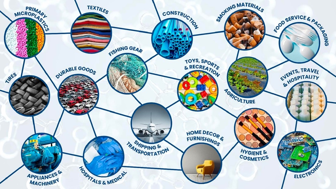
Today plastics are used throughout society. Erdle and Eriksen (2023) propose 17 sectors of plastic consumption, many of which have the potential to enter waterways and deposit into the ocean.
Debris can find its way into the ocean through numerous pathways, both direct and indirect. Fishing gear, for example, can be lost, abandoned, or discarded at sea, posing threats to marine wildlife. Single-use plastics like bottles, utensils, and bags can drift downstream into the ocean due to improper waste management or runoff from landfills. Many, if not all, sources of marine debris also face the risk of breaking down via weathering into smaller particles (known as microplastics) that travel easily through the water and atmosphere. These plastics travel from the deep-sea floor to arctic snow, persist for decades in aquatic environments, and can act as vectors by absorbing heavy metals, pathogens, and other chemical additives (Dey et al., 2020). Plastics ingested by marine organisms can amplify through the food chain and pass to humans through the consumption of seafood (Dey et al., 2020).
As the widespread impacts of marine debris continue to be revealed little by little, interdisciplinary efforts are necessary to better understand how pollution acts in aquatic environments and the most effective solutions to pursue. Significant data collection and analysis can tell scientists and researchers how to best move forward, which can be communicated to policymakers and the public. Aerial surveys, as performed by the Anderson Cabot Center for Ocean Life’s Spatial Ecology, Mapping, and Assessment (EcoMap) team and as further discussed in this document, are important to understand the types of debris, their pathways, impacts on marine wildlife, and possible correlations with regional phenomenon (construction, shipping, etc.). The methods and data that follow will serve as an introductory examination into marine debris in Southern New England waters from 2017-2022.
Behind the scenes
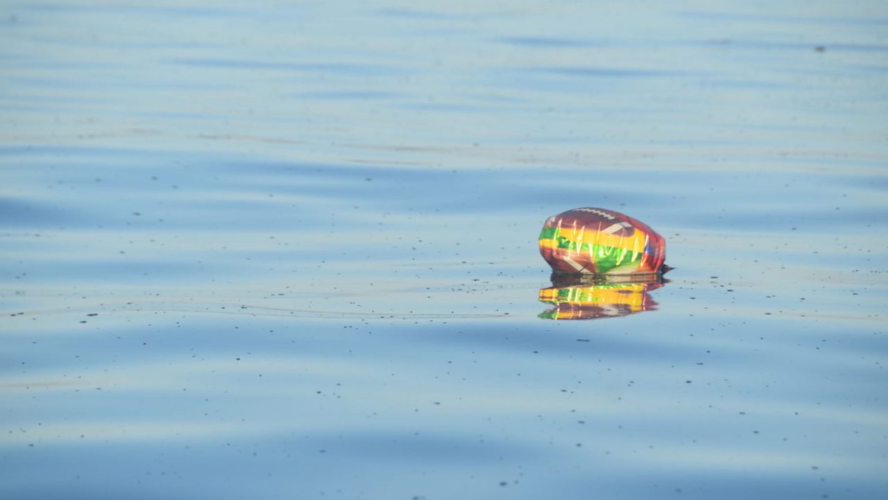
This work was performed as part of a summer marine debris internship with the Anderson Cabot Center for Ocean Life. All aerial survey images were previously collected over the course of several years by the EcoMap team and provided for this analysis (see an example in Appendix A).
Aerial survey images ranging from 2017-2023 were pre-assigned a debris code correlating to the type of pollution visible; the codes focused on in this work include DE-U (unidentified; this made up the majority of the images), DE-B (balloon), DE-P (plastic), DE-G (ghost gear), DE-R (rope) and DE-W (wood). All images were sorted by code, and details like the date and time, coordinates, size, and color of the debris were noted. This data was imported into ArcGIS Pro and plotted by debris location (see next section). Density estimates were then performed across each day, season, and year to identify any temporal trends. Lastly, Kruskal-Wallis tests— a method for testing whether samples originated from the same distribution—were performed to assess possible differences between seasons or years.
ArcGIS maps
The maps below represent the location of debris as imaged in southern New England waters from 2017–2023, across four seasons: winter (December–February), spring (March–May), summer (June–August), and fall (September–November). The grey line represents the survey region, and the purple shading represents wind energy lease areas. The dots are color-coded by year, and any pieces of debris that were coded as “DE-B” were marked with a star. Balloons—of the three debris codes used in this work—were specifically identified as they serve as a relatable reference object for the public.
The winter and spring months (Fig. 2 and 3) appeared to have the most debris, whereas the fall (Fig. 5) has the least. The reasoning for this has yet to be investigated, although potential margins for error include that not the same number of survey flights were conducted in each season year to year, and the 2023 data only includes images from the winter months, skewing the season as a whole.
-
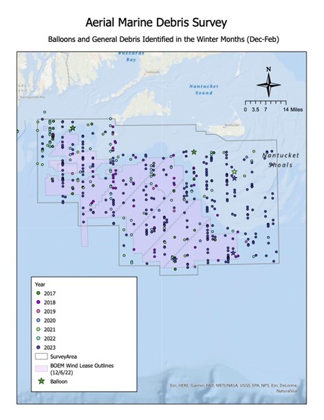
Fig 2. Marine debris in southern New England waters Documented via aerial survey, from 2017–2023 in December–February -
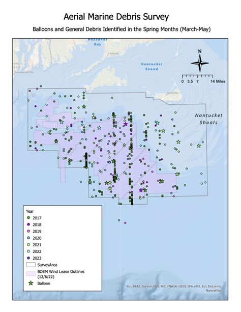
Fig 3. Marine debris in Southern New England waters Documented via aerial survey, from 2017–2023 in March–May -
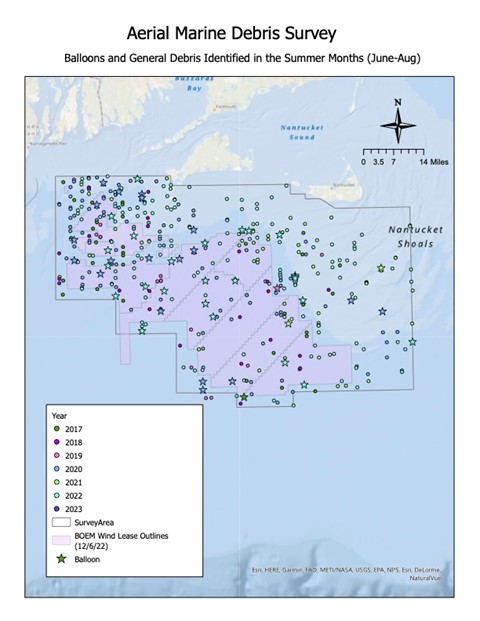
Fig 4. Marine debris in Southern New England waters Documented via aerial survey, from 2017–2023 in June–August -
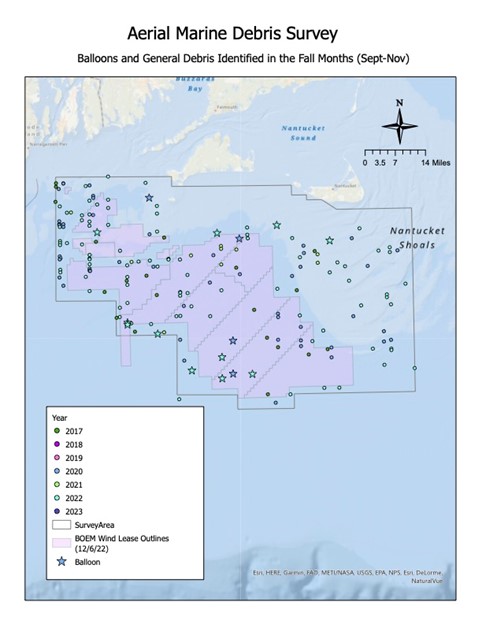
Fig 5. Marine debris in Southern New England waters Documented via aerial survey, from 2017–2023 in September–November
/
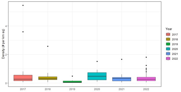
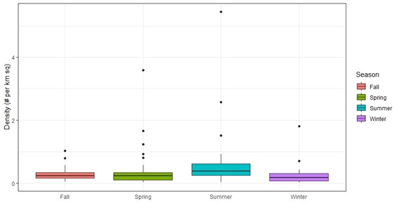
Density estimates and graphs
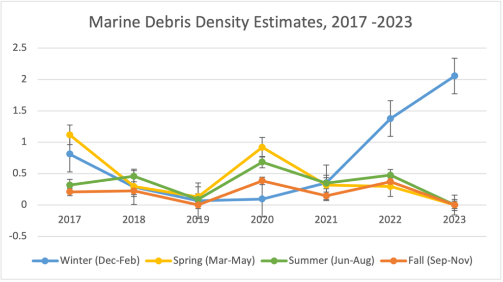
The two graphs below represent density estimates calculated in relation to the total number of aerial images taken. Calculations were run to determine density per day and per season across the range of years. Only debris codes DE-U, DE-B, and DE-P were included in this analysis as they were viewed as the most relevant (DE-W, or wood, for example, could be classified as debris or natural and was not considered a necessary addition here).
The first graph (Fig. 6) shows a consistently higher estimate in the spring and summer of each year, with a spike in the winter months beginning in 2021. While the reason for this is unknown, it’s important to recognize that, like with the ArcGIS maps, the only available 2023 data was for the winter months; this explains why, for the current year, winter has a high value, and the other three seasons remain at zero.
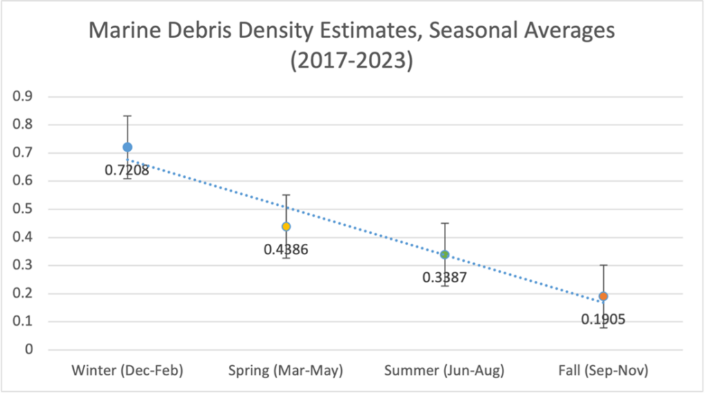
When each season was averaged across the years (Fig. 7), spring again ranks above summer, although both seasons place below winter. It is important to recognize, again, that the value for winter is significantly higher due to the imbalance of 2023 data that was used. Fall ranks as the lowest average, which makes sense when this graph is compared to the previous one.
Statistical analyses
In order to determine any statistically significant differences between density per year and per season, two Kruskal-Wallis tests were performed. It’s important to note that, unlike the ArcGIS maps and density estimates, the 2023 data was removed from these calculations, as only the winter months were available, and they noticeably skewed the results.
The Kruskal-Wallis test for density per year (Fig 8.) returned a p-value of 0.003116, which indicates statistically significant differences in density between years.
On the other hand, density per season (Fig. 9) returned a p-value of 0.03422, which shows some, but not convincing, evidence for a difference in density between seasons.
Together, the two tests show that there may be some temporal correlation for debris density, but this finding isn’t concrete. There are more significant differences in density when assessed by year, rather than by season, but still no clear pattern is visible, and further data collection and analysis is needed to draw solid conclusions.
Stay in the current
As previously discussed, marine debris is a global and growing pollution crisis with numerous sources at play and no singular best solution. Debris can spread quickly and widely through waterways and threaten aquatic wildlife, communities, and resources. This research not only provides a foundation for future marine pollution data collection, but it outlines next steps and recommendations as scientists and policymakers strive for solutions, both regionally and beyond.
Marine debris must also be taken down to the public level, as mass consumption drives improper waste management and increases the risk of pollution events. An important takeaway lies in purchasing habits, as plastic and single-use items are cheap, durable, and often readily available. Highlighting balloon debris in the above maps is a simple way to acknowledge the dangers of such a festive item—does every graduation, wedding, baby shower, and birthday need a bunch of balloons? Are there other items that are biodegradable or reusable that could be purchased instead? While the responsibility for mass consumption does lie on the producer, it also lies on the consumer, as habits and choices indicate a shift in societal values and trends. This research, both in its micro-focus on balloons and at large, provides a platform for public awareness and action.
Through the structure of this internship, preliminary involvement with policy development began with the creation of the first-ever NOAA Marine Debris Action Plan (MDAP) for Southern New England. While specific data from these surveys has yet to be shared with decision-influencing groups, general findings were shared in MDAP meetings, and this document will be offered up as a resource for future use.
Lastly, as exciting and novel as this work is, it only scratches the surface of the possibilities of aerial surveying work and the depth of the marine debris crises. The aerial images used in this research are taken from quite far away and only capture items large enough to be recognized from the and that float on or close to the surface. The data collected represents a minimum assessment, as there is significantly more debris unaccounted for of varying size and type.
Conclusion
This document functions as a guide to the work done by the Anderson Cabot Center for Ocean Life’s EcoMap team and is one resource in a sea of marine debris content. Everyone can play a role in reducing pollution, whether a member of the community, a scientist, a policymaker, a teacher; such a large-scale problem requires large-scale efforts and solutions—integrate conscious consumer choices daily, document pollution events, and amplify the voices committed to activism.
Our work is far from done.

Related Stories


Anderson Cabot Center for Ocean Life
Through pioneering marine conservation research and strategic partnerships, our team of 40 scientists works to combat the unprecedented impacts on the ocean from climate change and other human activities.